Security Analysis and Portfolio Management
Goal of the project:
The goal for this project was to analyze different securities and to form a portfolio. This project was for FINA 451 class at Colorado Mesa University. While creating a portfolio we had to follow an investment policy statement (IPS). This statement outlined the investor's (CMU's Finance and investment club) investment goals, risk tolerance, and other guidelines to follow.
Technologies used: Python, Excel, PowerPoint, python libraries: pandas, seasborn, yfinacne, matplotlib
How were the securities analyzed and portfolio formed?
The portfolio followed the guidelines of:
- Long term growth (5+ year outlook)
- Moderate risk tolerance
- NASDAQ and NYSE traded securities
- No financal derivaties
- Ethical securities that align with Daniels Fund Core Values
For each security we looked at:
- Beta (calculated based off S&P500 and the securities monthly return over a 5 year period)
- Expected Annual Return (Calculating using the Captial Asset Pricing Model or CAPM)
- Coeffient of Varation (Detererming a % representing risk:reward)
- Various other factors like Annual Dividend Yield, Market Share, Sector, and if the company has a positive community sentiment
Research:
Market Forces:
Researching and assessing different forces that can affect the market is important for investing. During the time of this project the key economic factors were interest rates and inflation. U.S. mortgage rates were at 7%, favoring the bond market. The U.S. inflation was at 3.7%, influencing higher purchasing power. There were also geopolitical events happening at the time. Most notably were the Russia/Ukraine and Israel/Palestine conflicts.
Sourcing the Securities Data:
Collecting each securities historical data was gathered by utilizing python and the yfinance library. Sourced by querying the needed historical price data from the Yahoo Finance API. This data was then exported as a CSV and imported into Excel.
Calculations:
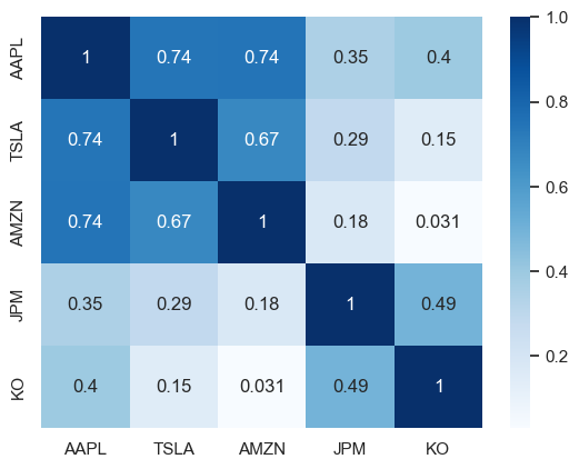
One of the calculations used was correlation represented by a correlation heat map. Correlation is important to research with a portfolio to determine if one security starts to take losses the others won't. This is determined by the difference of price changes between each security.
When the historical data was gathered, it was the daily market close price for the past 5 years. Outside of the correlation heatmap the monthly percent return was needed. Monthly Return = (Closing Price on Last Day of Month / Closing Price on Last Day of Previous Month) - 1. Once the monthly return was calculated for each security, finding the beta was next (Beta = Covariance/Variance). The beta represents the securities relation to the overall market(S&P 500 was used for the calculations). This can help determine risk and how each security moves with the market. Beta is considered high if > 1, low if < 1, and negative is < 0 meaning opposite correlation of the market. A high portion of securities that were examined had a high beta. It was determined this is because the S&P 500 has high holdings in the tech sector. Leading to the technology sector having a large influence on the overall market.
Capital Asset Pricing Model is widely used for expected returns (Ra = Rrf + [βa x (Rm – Rrf)]. This was the model chosen to use as it was a part of the classes curriculum along with it aligning with the other calculations used. CAPM has ease of use that was also a benefit. Each security that was researched had the CAPM performed on it. This gave an estimated return to use when determining the final portfolio holdings.
The last calculation used was Coefficient of Variation. This was used to evaluate the risk-to-reward of the security. This is a percentage form of how the standard deviation is related to the mean(S&P 500). The lower the Coefficient of Variation the less volatile or “risky” the security is.
Final Portfolio:
TThe Final portfolio had a Beta of 1.286, Expected Return of 9.13%, and a 21% Coefficient Variation (Risk:Reward). This portfolio had an asset allocation as follows: 70% stocks, 20% bonds, and 10% cash. The bond rates were at 5.2% which is very high, hence the large allocation in the portfolio.
Click here for the slides to the presentation